Simple Rabi oscillations

This tutorial shows how to set up the most basic two-level system and add a laser.

The top-level docstring becomes the intro text.

importing and initializing the System instance

from MoleCool import System, pi, plt

system = System('Rabi-2level') # description string

system.levels.add_electronicstate('g', 'gs') # ground electronic state
system.levels.g.add(F=0,mF=0) # add a single level with F=0

system.levels.add_electronicstate('e', 'exs') # excited electronic state
system.levels.e.add(F=1,mF=0) # add single mF=0 with F=1 as F=0 would be forbidden

System is created with description: Rabi-2level
/home/docs/checkouts/readthedocs.org/user_builds/molecool-py/checkouts/latest/MoleCool/Levelsystem.py:1573: UserWarning: Gamma must be defined for ElectronicState e! By default, it is now set to 1 MHz!
  warnings.warn(text)

The output shows a warning that no linewidth Gamma has been defined for the excited electronic state and thus the default value of 1 MHz is used for now.

Next, we can set the initial population to be completely in the ground state and define some quantities.

system.levels.g.set_init_pops({'F=0':1.0}) # initial population

ratio_OmGa  = 20 # ratio between Rabi frequency and the linewidth
Omega       = system.levels.calc_Gamma()[0] * ratio_OmGa # Rabi frequency
T_Om        = 2*pi/Omega # time of one period

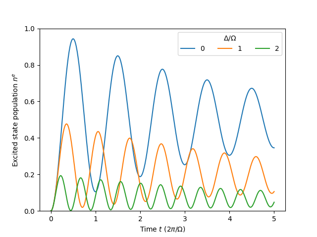
Evaluation and plotting

We now initialize the plot and add laser objects to the system. To iterate manually between different detunings of the laser, all laser objects are first reset at each iteration. Then the OBEs are propagated and the populations are plot against time.

fig = plt.figure(system.description)
plt.ylim([0,1])
plt.xlabel('Time $t$ ($2\pi/\Omega$)')
plt.ylabel('Excited state population $n^e$')

for det in [0,1,2]:
    del system.lasers[:] # delete laser instances in every iteration
    system.lasers.add(freq_shift = det*Omega/2/pi, freq_Rabi = Omega) # add laser component
    # or alternatively (using intensity instead of directly providing the Rabi freq.):
    # system.lasers.add(freq_shift = det*Omega/2/pi,
                      # I = 2*system.levels.Isat[0,0]*ratio_OmGa**2)

    system.calc_OBEs(t_int=5*T_Om, dt=1e-2*T_Om) # calculate dynamics with OBEs
    plt.plot(system.t/T_Om, system.N[1,:], label=str(det))

plt.legend(title='$\Delta/\Omega$',loc='upper right',ncols=3)

/home/docs/checkouts/readthedocs.org/user_builds/molecool-py/checkouts/latest/MoleCool/Levelsystem.py:293: UserWarning: There is no dipole matrix or reduced dipole matrix available!So a reduced matrix has been created only with ones:
exs     e
F       1
gs F
g  0  1.0
  warnings.warn(warn_txt)
Solving ode with OBEs...Execution time: 2.2742 seconds
Scattered Photons (e): 0.782994
Solving ode with OBEs...Execution time: 0.0036 seconds
Scattered Photons (e): 0.336916
Solving ode with OBEs...Execution time: 0.0048 seconds
Scattered Photons (e): 0.123428

<matplotlib.legend.Legend object at 0x799fb2c48070>