Getting started#
The user guide provides a more detailed walkthrough of MoleCool’s features and usage.
Code structure#
MoleCool is built in an object-oriented fashion. The toolbox offers
a streamlined workflow for initializing a System instance, enabling the
setup of laser beams, magnetic fields, and customizable multi-level systems.
For such configurations, the internal dynamics of a particle with complex
light fields can be computed via the rate equations or the OBEs.
The following diagram illustrates the code structure of the core classes.
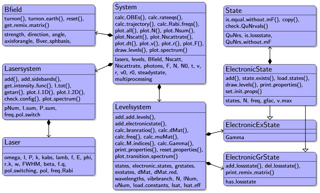
Class diagram of the core classes and their relationships of MoleCool,
where class composition is marked by arrows with diamonds and
class inheritance by open arrow tip.
Methods of individual classes are shown with parentheses, while
attributes and properties are labeled without them.#
System class#
The class System defines the central simulation
environment. It stores all information about the laser setup, the magnetic
field, the particle’s level structure, position and velocity as well as
computed quantities such as populations or trajectories.
Thus, creating the central interface for defining a physical setup typically
starts with creating an object of System.
from MoleCool import System
system = System(description='my_first_test', load_constants='138BaF')
During this initialization of the System object, single instances of
Levelsystem, Lasersystem and Bfield are created automatically and can
be accessed via the following attributes:
# Access its subsystems
print(system.lasers)
print(system.levels)
print(system.Bfield)
Lasersystem class#
The class Lasersystem defines the entire laser setup,
consisting of multiple beams with optional frequency sidebands.
The basic method add() constructs
the laser system from single Laser instances.
The method add_sidebands() is a
wrapper for conveniently adding multiple frequency sidebands.
# single laser at 860 nm with linear polarization and 20 mW of power:
system.lasers.add(
    lamb = 860e-9, P = 20e-3, pol = 'lin',
    )
# multiple laser objects with circular polarization are added at once
system.lasers.add_sidebands(
    lamb = 860e-9, P = 10e-3, pol = 'sigmap',
    sidebands = [-1, 0, 1],      # zero and first-order sidebands
    offset_freq = 20e6,          # common offset frequency of 20 MHz
    mod_freq = 40e6,             # modulation frequency of 40 MHz
    )
print(system.lasers)
Each Laser object stores its parameters (power, wavelength, polarization,
beam width, etc.) which can be accessed by indexing the Lasersystem object:
la = system.lasers[-1]   # save last added Laser object as a new variable
print(la)                # print laser properties
To remove lasers, use normal Python indexing:
del system.lasers[-1]     # delete last laser
del system.lasers[:]      # delete all lasers
Tip
Also explore other methods of Lasersystem,
such as visualization tools:
plot_spectrum(),
plot_I_1D(), or
plot_I_2D().
Each class can also be used independently for exploratory analysis
from MoleCool import Lasersystem

lasers = Lasersystem()
lasers.add(lamb=860e-9, P=20e-3, pol='lin')

print(lasers)
lasers.plot_I_1D()
or simply for calculating the intensity of a laser with given power and full width at half maximum (FWHM):
from MoleCool import Laser
print('Intensity in W/m^2:', Laser(P = 20e-3, FWHM = 5e-3).I)
print('Power in W:',         Laser(I = 700, FWHM = 5e-3).P)
Levelsystem class#
The class Levelsystem organizes all electronic (ElectronicState)
and other quantum states (State), allowing customizable and
interactive modifications of multi-level systems and their properties.
An instance of Levelsystem generally consists of several electronic states
ElectronicState – one electronic ground state
(ElectronicGrState) and multiple electronic
excited states (ElectronicExState).
An excited state features a natural lifetime / linewidth and decays into a
ground state, which may include a universal loss channel.
In the following example, the well-known \(D_2\) transition
\(5^2S_{1/2} \rightarrow 5^2P_{3/2}\) in rubidium \(^{87}\text{Rb}\)
is constructed with the lifetime \(\Gamma = 2 \pi \cdot 6.065\) MHz.
Subsequently, hyperfine levels as individual State objects with quantum
numbers (J, F, mF, etc.) are added to each electronic state.
from MoleCool import Levelsystem
# initiate empty level system
levels = Levelsystem()

# add electronic ground ('gs') and excited ('exs') state
levels.add_electronicstate('S12', 'gs')
levels.add_electronicstate('P32', 'exs', Gamma = 6.065)

# add single quantum states
levels.S12.add(J = 1/2, F = [1,2])
levels.P32.add(J = 3/2, F = [0,1,2,3])

# print all defined states with their quantum numbers
print(levels)
# this basically iteratively calls e.g.
print(levels.S12)
print(levels.S12[0])
Specific electronic or quantum states can also be removed from the level system:
levels.add_electronicstate('D52', 'exs', Gamma = 1.0)
del levels['D52']  # delete complete electronic state
del levels.P32[0] # delete first State object within P32
Note
States can only be added or deleted before any level-system property is initialized.
This combined level system features several physical properties required to simulate internal dynamics when interacting with light fields.
These properties, partly computable using the spectra module (see below),
include:
the electric dipole matrix and branching ratios (
dMat,dMat_red,vibrbranch)transition frequencies (
wavelengths,freq)magnetic g-factors (
gfac)lifetimes of the excited states (
Gamma)the mass of the particle (
mass)
Tip
To display all these properties, use
print_properties():
levels.print_properties() # or system.levels.print_properties()
For an empty level system, these properties are automatically generated
and can simply be modified using the internal pandas.DataFrame objects:
# set wavelengths in nm
levels.wavelengths.loc[('S12'), ('P32')] = 780.241
# same as normal array indexing:
# levels.wavelengths.iloc[:,:] = 780.241

# modify single entry of reduced electric dipole matrix
levels.dMat_red.loc[('S12', 1/2, 2), ('P32', 3/2, 0)] = 0
print(levels.dMat_red)

# modify first element of each the magnetic g-factor and frequency
# belonging to certain electronic states:
levels.S12.gfac.iloc[0] = 0.1234
levels.S12.freq.iloc[0] = -4.272

levels.P32.freq.loc[('P32', 3/2, 1)] = 10.
print(levels.P32.freq)

levels.print_properties()
As a convenient alternative, these properties can also be imported from a
.json file. Such a file can be created using the spectra module (see
below) via export_OBE_properties(),
or by using available data of various diatomic speciees from the repository’s
json files.
In this case, the electronic states are added as usual, and the remaining quantum states (matching optional quantum numbers) can be loaded directly from the json file, while all physical properties are imported automatically.
system = System(description='my_first_test', load_constants='138BaF')

# adding electronic states X and A
system.levels.add_electronicstate('X', 'gs')
system.levels.add_electronicstate('A', 'exs')

# loading all available states that match the provided quantum numbers v
system.levels.X.load_states(v=[0,1])
system.levels.A.load_states(v=[0])

print(system.levels)
Tip
Also check out other methods of Levelsystem and ElectronicState,
such as plotting the transition spectrum via
plot_transition_spectrum(),
setting initial population distributions via
set_init_pops(),
or plotting level diagrams via
draw_levels().
Bfield Module#
The class Bfield describes the magnetic field.
Every System instance contains a default zero field. A static, uniform field
with a strength of 5 G and an angle of 60 degrees relative to the z-axis
can be set up easily via:
system.Bfield.turnon(
    strength  = 5e-4,
    direction = [0, 0, 1],
    angle     = 60
    )
The magnetic field can be reset to zero at any time with
system.Bfield.reset().
Internal dynamics computation#
The internal dynamics of a system are governed by a set of coupled ordinary
differential equations (ODEs), solved using
scipy.integrate.solve_ivp().
Since these equations are evaluated repeatedly during simulations, MoleCool
compiles them into optimized machine code using numba’s just-in-time (JIT)
compiler, achieving performance comparable to C or FORTRAN.
For the rate-equation model calc_rateeqs(),
even long single-particle trajectories through multiple Gaussian laser beams
remain computationally efficient.
The adaptive LSODA integrator provides excellent stability and performance,
making it well suited for large-scale Monte Carlo simulations of particle
motion in realistic laser intensity profiles.
In contrast, solving the Optical Bloch Equations (OBEs)
calc_OBEs() typically relies
on explicit Runge–Kutta solvers such as RK45 (order 5).
Because OBE-based trajectory modeling requires precomputing quasi-steady-state
forces over various parameter combinations, these simulations are more
computationally demanding. To mitigate this, MoleCool employs Python’s
multiprocessing module to parallelize independent simulations across
multiple CPU cores, significantly reducing total runtime.
Performance and Parallelization#
Dynamics equations are solved with
scipy.integrate.solve_ivp()and JIT-compiled withnumbafor high efficiency.The
multiprocessingmodule parallelizes independent runs across available CPU cores, enabling extensive parameter sweeps and faster convergence of Monte Carlo statistics.
Example: Optical cycling simulation for BaF#
from MoleCool import System
import numpy as np

system = System(description='SimpleTest1_BaF', load_constants='138BaF')

# Define lasers with multiple sidebands
for lamb in np.array([859.830, 895.699, 897.961]) * 1e-9:
    system.lasers.add_sidebands(lamb=lamb, P=20e-3, pol='lin',
                                offset_freq=19e6, mod_freq=39.33e6,
                                sidebands=[-2, -1, 1, 2],
                                ratios=[0.8, 1, 1, 0.8])

# Load all relevant vibrational states
system.levels.add_all_levels(v_max=2)

# Run a rate-equation simulation
system.calc_rateeqs(t_int=20e-6)

# Plot populations and forces
system.plot_N()
system.plot_F()
system.plot_Nscatt()
Note
Rate equations are highly efficient for long trajectories and can be
integrated with LSODA, while OBEs use explicit Runge–Kutta methods (RK45).
Both solvers are JIT-compiled with numba for near-C performance.
Other modules#
spectra module#
The module spectra provides an independent toolset for
computing molecular spectra.
It handles effective Hamiltonians and spectral analysis to extract
physical properties – such as branching ratios and transition frequencies –
(and can export them to .json files) as required for simulating internal
dynamics using the optical Bloch equations or a rate-equation model.
The following snippet outlines how to calculate a simple spectrum for
\(^{138}\text{BaF}\). See the extensive example
Spectrum RaF for more details and
features of the spectra module.
from MoleCool.spectra import ElectronicStateConstants, Molecule, plt

# defining spectroscopic constants
const_gr = ElectronicStateConstants(const={
    'B_e' : 0.2159,   'D_e' : 1.85e-7,  'gamma' : 0.0027,
    'b_F' : 0.0022,   'c'   : 0.00027,
})
const_ex = ElectronicStateConstants(const={
    'B_e' : 0.2117,   'D_e' : 2.0e-7,   'A_e' : 632.2818,
    'p'   : -0.089545,'q'  : -0.0840,
    "g'_l": -0.536,   "g'_L":0.980,
    'T_e' : 11946.31676963,
})

# initiating empty Molecule instance and adding electronic states
# with all quantum states up to a certain quantum number F
BaF = Molecule(I1 = 0.5, mass = 157, temp = 4)
BaF.add_electronicstate('X', 2, 'Sigma', const=const_gr)
BaF.add_electronicstate('A', 2, 'Pi', Gamma=2.84, const=const_ex)
BaF.build_states(Fmax=8)

# calculating branching ratios and molecular spectrum
BaF.calc_branratios()
E, I = BaF.calc_spectrum(limits=(11627.0, 11632.8))

# plotting
plt.figure()
plt.plot(E, I)
plt.xlabel('Frequency (cm$^{-1}$)')
plt.ylabel('Intensity (arb. u.)')
This workflow enables independent analysis of molecular spectra, extraction of constants, and direct feedback into the simulation modules.
tools module#
The module tools provides a versatile collection of utility
functions and helper routines that extend the capabilities of the
MoleCool toolbox.
saving and loading JSON files and Python objects (
save_object(),open_object(), andget_constants_dict())managing large-scale internal dynamics evaluations across multidimensional parameter or configuration spaces using Python’s
multiprocessingmodulecomputing data and save it as arrays (
multiproc())retrieving and plotting selected results (e.g., force profiles) in a convenient way (
get_results(),plot_results())
converting between temperatures, velocities, and Gaussian widths (
FWHM2sigma(),vtoT(),gaussian(), etc.)definitions of various differential equations (
ODEs)computing and evaluating simple linear trajectories through multiple apertures (
diststraj)
Next Steps#
Once you are familiar with the core workflow, continue with the complete
tutorial in the Examples section to explore additional
functionalities of MoleCool and apply them to real-world examples using
advanced workflows.