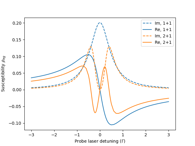
EIT

This examples employs a 3-level system to show the effect of EIT.

EIT (electromagnetically-induced transparency).

Import

from MoleCool import System, np, plt, pi

det_pump = 0*1e6 # pump laser detuning for for EIT resonance position in Hz
I_probe  = 0.2 # laser intensity of probe beam in W/m^2
I_pump   = 5.0 # laser intensity of pump beam in W/m^2
gr_split = 1000 # splitting between both ground states in MHz

Calculation routine

Deltas  = np.array([*np.arange(-3,-0.5,0.1),*np.arange(-0.5,0.,0.01)])*1e6
Deltas  = np.array([*Deltas,*(-np.flip(Deltas[:-1]))]) + det_pump

rho     = np.zeros((2,len(Deltas)),dtype=complex) # steady state density matrix elements
for i in range(2):
    system = System('testingEIT')
    system.levels.add_electronicstate('e', 'exs') # first add only excited state
    system.levels.e.add(F=1,mF=0) # add single mF=0 with F=1 as F=0 would be forbidden

    # simple two-level case:
    if i == 0:
        system.levels.add_electronicstate('g', 'gs') # ground electronic state
        system.levels.g.add(J=0.5,F=0,mF=0) # add a single level with F=0
        # initial population can be specified but makes no difference for steady state
        system.N0 = [1,0]

    # Lambda-level scheme for EIT case:
    if i == 1:
        system.levels.add_electronicstate('g', 'gs') # ground electronic state
        system.levels.g.add(J=0.5,F=0,mF=0) # add two single levels with F=0
        system.levels.g.add(J=1.5,F=0,mF=0)
        system.levels.g.freq.iloc[1] = -gr_split # detuning in MHz between both ground states

    # Iterating over all detunings of scanning probe laser:
    for j,Delta in enumerate(Deltas):
        del system.lasers[:] # delete laser instances in every iteration
        system.lasers.add(I=I_probe, freq_shift=Delta) # (weak) probe laser
        # only add pump laser for EIT case:
        if i == 1:
            system.lasers.add(I=I_pump, freq_shift=+gr_split*1e6+det_pump)

        T_Om = 2*pi/np.abs(system.calc_Rabi_freqs()).max() # period time of Rabi frequency
        # calculate dynamics until steady state is reached
        system.calc_OBEs(t_int=5*T_Om, steadystate=True, verbose=False)

        # transform density matrix elements (ymat) to the other rotating frame
        # which rotates with level's transition frequency instead laser frequency
        rho[i,j] = (system.ymat[0,-1,:] * np.exp(1j*system.t*Delta*2*pi)).mean()

System is created with description: testingEIT
/home/docs/checkouts/readthedocs.org/user_builds/molecool-py/checkouts/stable/MoleCool/Levelsystem.py:1573: UserWarning: Gamma must be defined for ElectronicState e! By default, it is now set to 1 MHz!
  warnings.warn(text)
/home/docs/checkouts/readthedocs.org/user_builds/molecool-py/checkouts/stable/MoleCool/Levelsystem.py:293: UserWarning: There is no dipole matrix or reduced dipole matrix available!So a reduced matrix has been created only with ones:
exs         e
F           1
gs J   F
g  0.5 0  1.0
  warnings.warn(warn_txt)
System is created with description: testingEIT
/home/docs/checkouts/readthedocs.org/user_builds/molecool-py/checkouts/stable/MoleCool/Levelsystem.py:1573: UserWarning: Gamma must be defined for ElectronicState e! By default, it is now set to 1 MHz!
  warnings.warn(text)
/home/docs/checkouts/readthedocs.org/user_builds/molecool-py/checkouts/stable/MoleCool/Levelsystem.py:293: UserWarning: There is no dipole matrix or reduced dipole matrix available!So a reduced matrix has been created only with ones:
exs         e
F           1
gs J   F
g  0.5 0  1.0
   1.5 0  1.0
  warnings.warn(warn_txt)

Plotting results

plt.figure('Susceptibility')
for i,case in enumerate(['1+1','2+1']):
    plt.plot(Deltas*1e-6,rho[i].imag,'--',label=f"Im, {case}", c='C'+str(i))
    plt.plot(Deltas*1e-6,rho[i].real,'-',label=f"Re, {case}", c='C'+str(i))

plt.xlabel('Probe laser detuning ($\Gamma$)')
plt.ylabel('Susceptibility $\\rho_{eg}$')
plt.legend(loc='upper right')

<matplotlib.legend.Legend object at 0x72ede43ed390>