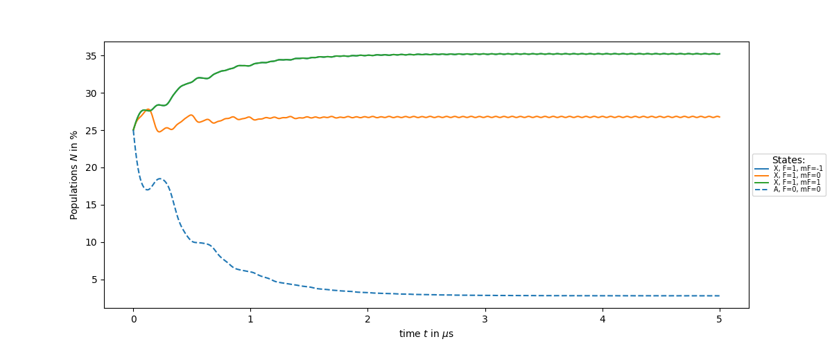
Simplest type-II levelsystem

creating 3+1 level system and observing time-dependent populatios.

System is created with description: Simple3+1
****************************************
************* Levelsystem **************
****************************************

mass (in u): 0.0

++++++++++++ level-specific ++++++++++++

-------------------X--------------------

g-factors:
gs  F
X   1    0.0
dtype: float64

frequencies (in MHz):
gs  F
X   1    0.0
dtype: float64

-------------------A--------------------

g-factors:
exs  F
A    0    0.0
dtype: float64

frequencies (in MHz):
exs  F
A    0    0.0
dtype: float64

Gamma (in MHz):
exs A 1.0

+++++++++ transition-specific ++++++++++

transition dipole moments:
     A
X  1.0

-----------------X <- A-----------------
/home/docs/checkouts/readthedocs.org/user_builds/molecool-py/checkouts/v3.7.1/MoleCool/Levelsystem.py:293: UserWarning: There is no dipole matrix or reduced dipole matrix available!So a reduced matrix has been created only with ones:
exs     A
F       0
gs F
X  1  1.0
  warnings.warn(warn_txt)

dipole matrix:
exs            A
F              0
mF             0
gs F mF
X  1 -1  0.57735
      0 -0.57735
      1  0.57735

vibrational branching:
exs    A
gs
X    1.0

wavelengths (in nm):
exs       A
F         0
gs F
X  1  860.0
Solving ode with OBEs...Execution time: 1.8978 seconds
Scattered Photons (A): 1.569080

from MoleCool import System

system = System(description='Simple3+1') # create empty system instance first

# construct level system:
# - create empty instances for a ground and excited electronic state
system.levels.add_electronicstate(label='X', gs_exs='gs')
system.levels.add_electronicstate(label='A', gs_exs='exs', Gamma=1.0)
# - add the levels with the respective quantum numbers to the electronic states
system.levels.X.add(F=1)
system.levels.A.add(F=0)
# - next all default level properties can be displayed and simply changed
system.levels.print_properties()
system.levels.X.gfac.iloc[0] = 1.0 # set ground state g factor to 1.0

# set up lasers and magnetic field
system.lasers.add(lamb=860e-9, P=5e-3, pol='lin') #wavelength, power, and polarization
system.Bfield.turnon(strength=5e-4, direction=[0,1,1]) #magnetic field

# simulate dynamics with OBEs and plot population
system.calc_OBEs(t_int=5e-6, dt=10e-9, magn_remixing=True, verbose=True)
system.plot_N()